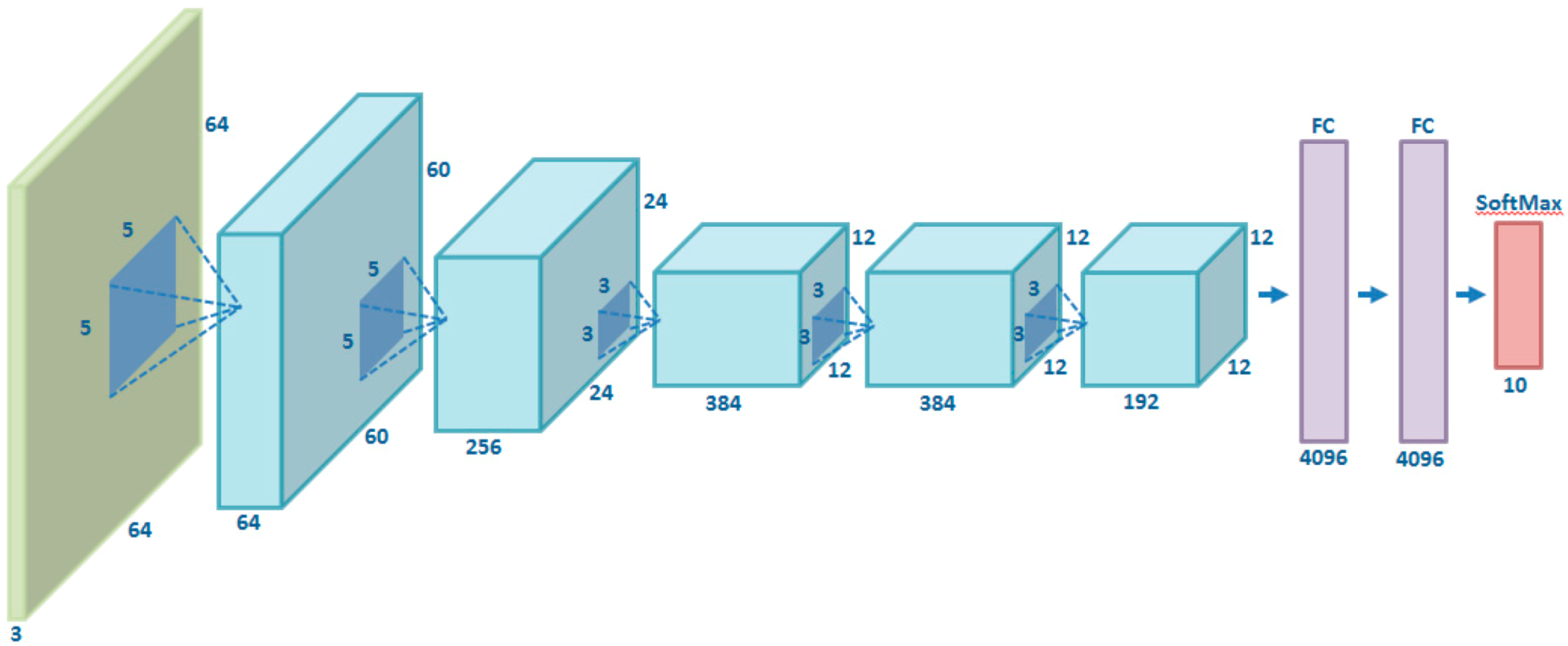
A CNN is pretrained for image classifications (e.g. ImageNet) and one of its intermediate layers is used as a feature extractor
A region proposal network (RPN) finds up to a predefined number of regions
Initially all combinations of given sizes (e.g. 64, 128, 256 pixels) and given ratios between width and height (e.g. 0.5, 1.0, 1.5) are used as reference regions
RPN learns to predict a probability that a reference region contains an object, and x, y, width, and height offset from the reference
The extracted features are reused for classifying the regions using a region-based CNN (R-CNN)
R-CNN consists of two fully-connected layers of size 4096, followed by two output layers—one predicting the class (including “background”) and one predicting the region offset
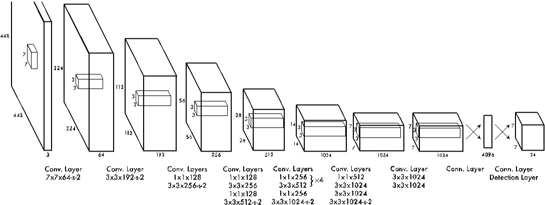
A single convolutional network extracts features and predicts the bounding boxes
The input image is conceptually divided into a grid of cells (for example, 7 × 7)
For each cell, the model predicts multiple bounding boxes (for example, two), whose center falls into the cell, and one set of class probabilities
The model predicts 5 values for each bounding box:
x and y coordinates (between 0 and 1, relative to the cell)
width and height (between 0 and 1, relative to the image)
confidence score (between 0 and 1)
At test time, the confidences are multiplied by the class probabilities to get a set of class scores for each bounding box
For every bounding box, keeps only the class with the highest score
Overlapping bounding boxes are filtered using non-maximum suppression
At training time, the bounding box with the highest Intersection over Union with a ground truth bounding box is “responsible for predicting the object”, i.e. takes part in the loss calculation
Target for the confidence score is the Intersection over Union between the predicted and ground truth bounding boxes
The loss of a bounding box is the sum of squared errors from its coordinates and dimensions, confidence score, and class probabilities
There are multiple detection layers at different levels of the model (for example, 3)
Each grid cell at each detection layer predicts multiple bounding boxes (for example, 3) and a separate set of class probabilities for every box (as opposed to YOLO)
Boxes are predicted relative to predefined anchor boxes, like in Faster R-CNN
The anchor boxes are centered at the cell center, i.e. the bounding box location is still predicted relative to the grid cell and the anchor box only defines a prior width and height
The three boxes predicted at a cell each have a separate prior width and height
The three detection layers use separate priors, totaling nine anchor box shapes
The anchor box dimensions are determined by running k-means clustering on the training set bounding boxes
At each detection layer, the bounding box that is responsible for a training target is the one whose anchor box best matches the object
The grid cell is determined by the object center
The predictor within the cell is the one whose prior dimensions give the ighest Intersection over Union with the target
Confidence score is now called objectness, and YOLOv3 uses binary targets
The target is one for the bounding boxes that are responsible for predicting any objects
Bounding boxes that are not responsible for predicting any objects, but whose anchor box overlaps an object (high enough IoU), are ignored from the objectness loss
Objectness loss is calculated as the binary cross entropy from those boxes that are not ignored
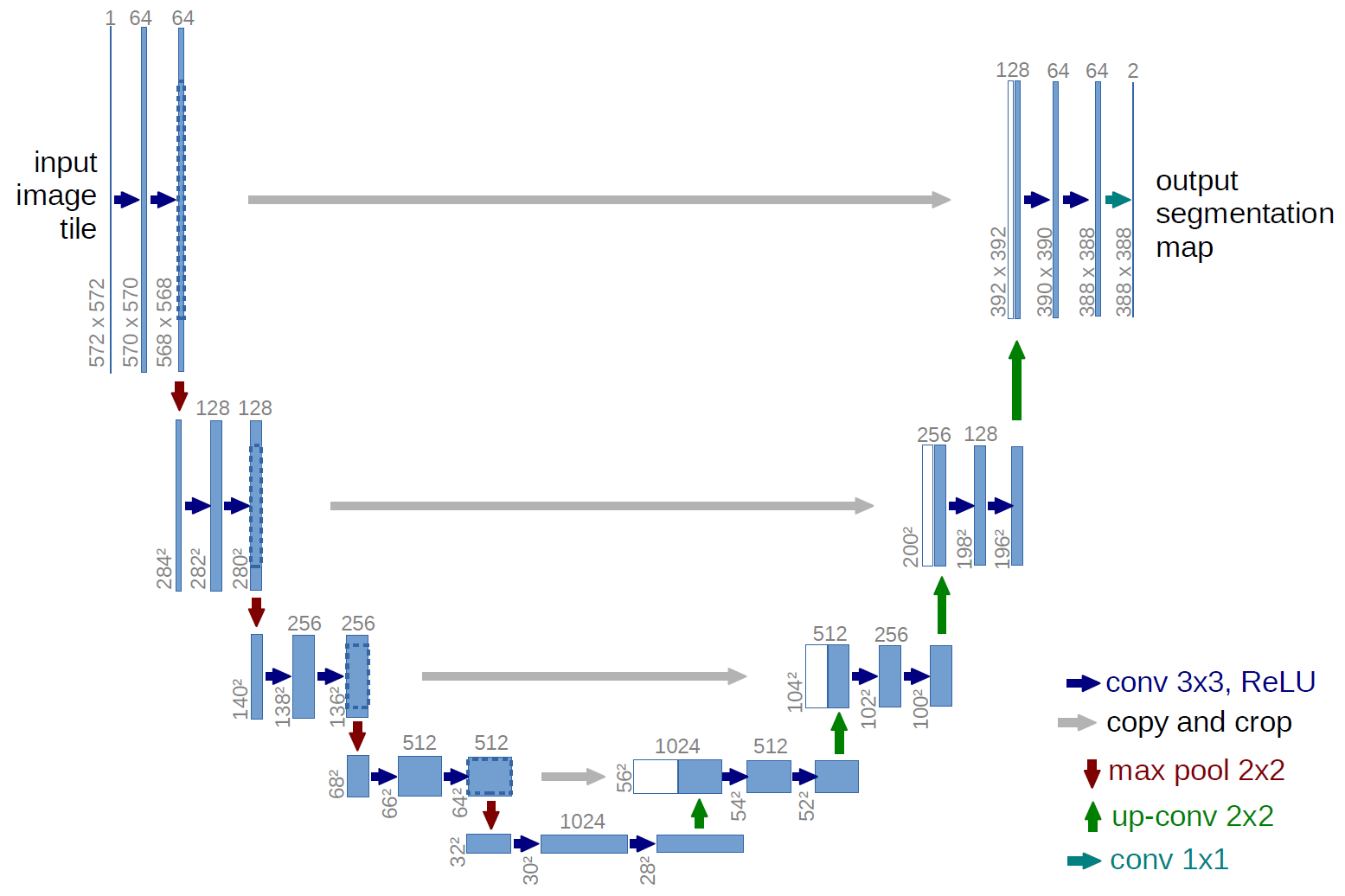
After reducing resolutiong using the usual convolutional layers, increase the resolution by upsampling
Cross connections (not part of the original U-Net architecture) from the downsampling part of the network to the same-sized image in the upsampling part