Understanding convergence of SGD

Batch size, learning rate, weight averaging, and solutions that generalize better

References

This article discusses several papers that I recently found, that analyze stochastic gradient descent optimization, make interesting observations about its convergence, and help understanding the significance of batch size and learning rate:

• McCandlish et al. 2018. An Empirical Model of Large-Batch Training.
• Keskar et al. 2017. On Large-Batch Training for Deep Learning: Generalization Gap and Sharp Minima.
• Smith and Le 2018. A Bayesian Perspective on Generalization and Stochastic Gradient Descent.
• Smith et al. 2018. Don’t Decay the Learning Rate, Increase the Batch Size.
• Izmailov et al. 2018. Averaging Weights Leads to Wider Optima and Better Generalization.

Training batch size

Stochastic gradient descent (SGD) is basically gradient descent using noisy gradients of the training loss. The batch size determines the quality of the gradient estimates. The gradient being calculated as an average over the examples in a mini-batch, its variances scales inversely with the batch size. The more examples that are being used to estimate the gradient, the more accurate the estimates are.

Given that the different examples in a mini-batch can be processed in parallel in a GPU, it seems to be a good idea to use as large batch size as possible. The assumption is that this makes the training converge faster. Also the Transformer model especially requires large enough batch size to converge at all. In theory we could always increase the batch size by using more GPUs. However, when the gradient estimates get closer to the true gradient, at some point increasing the batch size will barely improve the model update anymore. The increased communication between the GPUs would also reduce the possible gains in terms of training speed.

How should we then choose the batch size in order to train as efficiently as possible? The next section tries to quantify the noise introduced to gradient estimates by using a specific batch size, and its impact on the progress that a training step can make.

Optimal learning rate and saturation of gradient estimates

At each step SGD moves the model parameters $\theta$ towards the negative gradient an amount specified by the learning rate or step size $\epsilon$. Optimal step size would of course be one that minimizes the new loss $L(\theta - \epsilon G)$. McCandlish et al. show how we could estimate the optimal step size if we had access to the true gradient $G$ and the true Hessian $H$. They approximate the new loss using the second-order Taylor expansion. The second-order Taylor expansion of function $f(x)$ with a real argument can be written

$$ f(a + x) \approx f(a) + x f'(a) + \frac{1}{2} x^2 f''(a). $$

In the same way we can approximate the new loss. We’ll just write it in matrix form:

$$ L(\theta - \epsilon G) \approx L(\theta) - \epsilon G^T G + \frac{1}{2} \epsilon^2 G^T H G $$

This function can be minimized by setting the derivative to zero. This gives the optimal step size for the true gradient:

$$ \epsilon_{max} = \frac{\left|G\right|^2}{G^T H G}. $$

Using this to estimate the learning rate at each step would be very costly, since it would require the computation of the Hessian matrix. In fact, this starts to look a lot like second-order optimization, which is not used in deep learning applications because the computation of the Hessian is too expensive. However, now we’re just trying to understand what happens to the optimal learning rate and batch size under noise.

When using SGD with batch size $B$, the gradient estimates are noisy and we need to consider the expectation of $L(\theta - \epsilon G)$. McCandlish et al. also derive the optimal step size in this case, which can be expressed:

$$ \epsilon_{opt}(B) = \frac{\epsilon_{max}}{1 + B_{noise} / B} $$

They call the quantity $B_{noise}$ the gradient noise scale. The noise scale depends on the true gradient and Hessian, and the variance of the gradient.

Some observations they make about the noise scale:

• One would expect it to be larger for difficult tasks, where examples are less correlated.
• It doesn’t depend on the size of the data set. Model size shouldn’t have much effect either.
• During training the magnitude of the gradient decreases, so the noise scale grows.

There is a similar relation between the best possible improvement in loss with true gradient, $\Delta L_{max}$, and the best possible improvement under noise, $\Delta L_{opt}(B)$:

$$ \Delta L_{opt}(B) = \frac{\Delta L_{max}}{1 + B_{noise} / B} $$

Some interesting points that are made about selecting batch size and learning rate:

• As larger batch sizes give better gradient estimates, a larger learning rate can be used.
• There’s a good chance the training will diverge when the step size is larger than twice $\epsilon_{opt}$.
• When the batch size is a lot smaller than $B_{noise}$, increasing batch size linearly increases the progress in loss.
• When the batch size is a lot larger than $B_{noise}$, increasing batch size has hardly any effect on the progress.

Flat minima generalize better

Intuitively it’s easy to understand that larger batches lead to faster convergence, but after certain point growing the batch size doesn’t really help anymore. However, this doesn’t explain the well known fact that a too large batch size can even hurt the model performance. Keskar et al. observed that large batches yield a similar training loss, but generalize worse than small-batch training. They found two reasons for the worse generalization performance:

• Large-batch training tends to converge to a minimum close to the initial parameter values, instead of exploring all the parameter space.
• Large-batch training tends to converge to sharper minima, while small-batch training converges to flatter minima.

They illustrate the generalization capability of flat and sharp minima using a loss function $f(x)$ with only a single parameter $x$:

Generalization capability of a flat and a sharp minimum. Keskar et al.

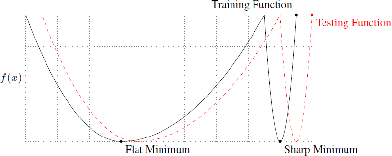
Both minima reach the same loss value, but the flat minimum is less sensitive to perturbations in the parameter space. They provide experimental evidence that large-batch training converges more likely to sharp minima and minima close to the starting point. They argue that the inherent noise in small-batch training helps to push the parameters out of a sharp basin.

Useful random fluctuations

McCandlish et al. looked at how noise degrades gradient estimates and found a point of diminished returns for batch size. In Appendix C they make an empirical observation that the noise scale primarily depends on the learning rate and batch size, and under some assumptions is approximately proportional to $B / \epsilon$. Their definition of the noise scale is independent of the training set size.

Smith and Le observed that some amount of noise is helpful, so there is an optimal value for batch size, when other hyperparameters are kept fixed. They try to assess the noise level in SGD by interpreting it as integration of a stochastic differential equation. With true gradient $d C / d \omega$ the gradient descent update can be written

$$ \Delta \omega = - \frac{\epsilon}{N} \frac{d C}{d \omega}, $$

where normalization by the training set size $N$ comes from the fact that we define the cost as the sum of the costs from individual training examples, but in practice we want to take the average. When estimating the gradient from a mini-batch, an error term must be added. They write this as a stochastic differential equation

$$ \frac{d \omega}{d t} = - \frac{d C}{d \omega} + \eta(t), $$

where $\eta(t)$ represents noise. Integrating this equation over the span of $\epsilon / N$ represents one SGD update.

They calculate the variance in the update in two ways and equate them: from the discrete equation, assuming Gaussian gradient noise, and from the differential equation, by integrating $\eta(t)$. This gives a formula for a “scaling factor” in the variance that they call the noise scale, $g \approx \epsilon N / B$. Assuming that there is an optimal scale of random fluctuations, $g$ should be kept fixed. This implies that the optimal batch size is proportional to $\epsilon N$. Similarly, when increasing batch size, learning rate should be increased proportionally.

So essentially a small batch size and a high learning rate serve the same purpose—increase the fluctuations that are helpful for learning. In this sense decaying learning rate during training is very similar to simulated annealing. A larger learning rate will explore a larger area of the parameter space, while decaying it will allow training to converge to a minimum. In another paper Smith et al. suggest to increase the batch size instead of annealing learning rate, which makes sense if there’s more GPU memory available than what the optimal batch size can initially utilize.

Averaging model parameters

A very interesting approach for finding flat minima was recently proposed by Izmailov et al.. Instead of continuously decaying the learning rate, it’s possible to find several different models by using a cyclical learning rate schedule. This means simply that the learning rate is repeatedly decayed to zero, and then raised again to a higher value. The model parameters are saved after each decay cycle. They observed that the model parameters traverse around the minimum, but never quite reaching the optimal point.

This suggests that an improved model can be obtained by taking the averages of the values of each parameter in the intermediate models. The figure below shows three intermediate models ($W_1, W_2, W_3$) and an average model ($W_{SWA}$) in the parameter space.

Three models obtained by training using cyclical learning rate, and an average model. Izmailov et al.

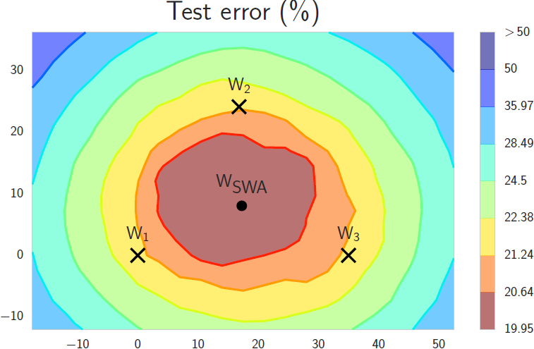
Izmailov et al. call this method stochastic weight averaging (SWA), and observe that the solutions found by SWA are broader in the sense that even if the training loss might be slightly higher, the model is not as sensitive to perturbations of the parameters. This improves the generalization of the model, with no extra cost, except for storing the intermediate models.