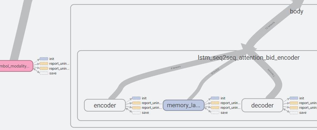
## Gentle Introduction to TensorFlow * Sessions * Variables * Broadcasting * Optimization * Devices * Recurrency * Debugging * TensorBoard --- ## Introduction * Numerous machine learning toolkits utilize the same principle—the user describes a neural network using a graph consisting of operations (forward pass) and the toolkit performs automatic differentiation (backward pass). * Theano, Torch, Keras, Caffe, CNTK, MXNet * Development is by far most active around TensorFlow. * Tensor2Tensor for sequence-to-sequence modeling. * C++ API can be used to execute graphs built using the Python API in a production environment. --- ## Basic Concepts * `tf.Graph` class represents a computation graph. * By default all operations and variables are placed in the default graph. * `tf.Tensor` represents the output of an operation. * `tf.Variable` represents persistent state. * `tf.Session` is a class for performing computation on a graph. * By default, the default graph is used. * Maintains the state of the variables between `run()` calls. ```python a = tf.constant(1.0) b = tf.constant(2.0) c = a + b sess = tf.Session() print(sess.run(c)) # 3.0 ``` --- ## Variables * Before using variables, they have to be initialized. * `init_op` sets them to the initial value given in the constructor. * Alternatively their state can be read from a *checkpoint* file. ```python a = tf.Variable(0.0) b = tf.constant(1.0) assign_op = tf.assign(a, a + b) init_op = tf.global_variables_initializer() sess = tf.Session() sess.run(init_op) print(sess.run(assign_op)) # 1.0 print(sess.run(assign_op)) # 2.0 ``` --- <!-- .slide: data-transition="fade-in none-out" --> ## Model Parameters * Usually model parameters are created using `tf.get_variable(name, shape)`. * "Traditional" way of constructing a layer is by creating a class. ```python class MyLayer(base.Layer): def __init__(self, units_in, units_out, name): self.kernel = tf.get_variable(name + "/kernel", shape=[units_in, units_out]) self.bias = tf.get_variable(name, + "/bias", shape=[units_out]) def __call__(self, input): return tf.matmul(input, self.kernel) + self.bias ``` --- <!-- .slide: data-transition="none-in none-out" --> ## Model Parameters * Most of the time another convention is used in TensorFlow. * Trainable variables are collected automatically. * `with tf.variable_scope()` is convenient for creating name hierarchies. * Makes debugging a lot easier. ```python def my_layer(input, units): kernel = tf.get_variable("kernel", shape=[inputs.get_shape()[1], units]) bias = tf.get_variable("bias", shape=[units_out]) return tf.matmul(input, kernel) + bias with tf.variable_scope(name): output = my_layer(input, units) ``` --- <!-- .slide: data-transition="none-in fade-out" --> ## Model Parameters * What if we want to apply the same layer to different inputs (without creating new weights)? ```python with tf.variable_scope(name): output1 = my_layer(input1, units) tf.get_variable_scope().reuse_variables() output2 = my_layer(input2, units) ``` --- ## Tensor Shape * `tensor.get_shape()` returns the static shape, known at compile time. * `tf.shape(tensor)` returns a Tensor that represents the dynamic shape. ```python batch_size = 16 length = tf.placeholder(tf.int32) inputs = tf.zeros((batch_size, length)) static_shape = inputs.get_shape() # TensorShape; (16, ?) dynamic_shape = tf.shape(inputs) # Tensor; [16, length] ``` --- <!-- .slide: data-transition="fade-in none-out" --> ## Broadcasting 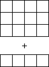 <!-- .element: class="plain" --> * Convert tensors to the same shape to make operations compatible. * Elementwise binary operations follow NumPy broadcasting. * The shape of the low-rank tensor must match the trailing dimensions of the high-rank tensor. --- <!-- .slide: data-transition="none-in fade-out" --> ## Broadcasting * Matrix multiplication `tf.matmul()` does not broadcast. The tensors have to be converted to 2D first. ```python x = tf.random_normal([i, j, k]) y = tf.random_normal([k, l]) x = tf.reshape(x, [-1, k]) z = tf.matmul(x, y) z = tf.reshape(z, [i, j, l]) ``` * Note that if you want a linear layer / multiplication by a weight matrix, it's easier to use `tf.layers.dense(x, size, use_bias=False)`. --- ## Optimization * Common optimization methods are implemented in various subclasses of `tf.train.Optimizer`. * AdadeltaOptimizer, AdagradOptimizer, MomentumOptimizer, AdamOptimizer * By default all *trainable* variables are optimized. * `minimize(cost)` returns an operation that performs one training step. ```python optimizer = GradientDescentOptimizer(learning_rate=0.1) optimizer_op = optimizer.minimize(cost) for i in range(training_steps): sess.run(optimizer_op) ``` --- ## Devices * An operation can run on a CPU (`"/cpu:0"`) or a GPU (`"/device:GPU:0"`). * By default, the first GPU device is selected, if the operation has a GPU implementation (and you have a GPU). * `with tf.device('/device:GPU:N')` assigns variables and operations to GPU `N`. * Setting configuration variable `log_device_placement=True` causes the device mapping to be printed. * By default, TensorFlow maps all memory of all GPUs. * Set `CUDA_VISIBLE_DEVICES=N` unless job scheduler is allocating a GPU for your process. --- <!-- .slide: data-transition="fade-in none-out" --> ## Recurrency * `RNNCell` is an abstract class that defines a recurrent layer as a function of activations and state. * Input, output, and state are 2-dimensional: `[sequences, units]` 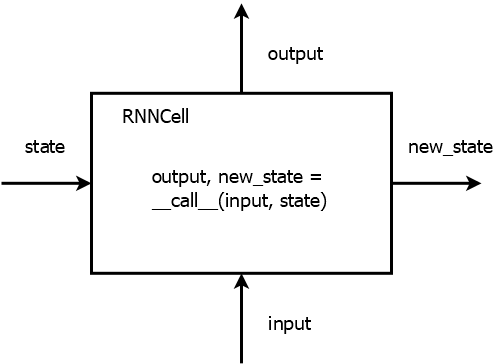 <!-- .element: class="plain" --> --- <!-- .slide: data-transition="none-in fade-out" --> ## Recurrency * There are several different RNN cells already implemented in `tf.contrib.rnn`: `LSTMCell`, `GRUCell`, ... * To insert a recurrent layer into a graph, use `tf.nn.dynamic_rnn(cell, inputs)`. * Inputs and outputs are 3-dimensional: `[sequences, time, units]` * Initial state can be given as input and final state is received as output (2-dimensional). ```python cell = tf.nn.rnn_cell.LSTMCell(num_units) outputs, final_state = tf.nn.dynamic_rnn(cell, inputs, initial_state) ``` --- <!-- .slide: data-transition="fade-in none-out" --> ## RNNCell Wrappers * Wrap some functionality over another RNN, e.g. `LSTMCell`. * `MultiRNNCell(cells)` * Stacks a list of RNNCells on top of each other. * State is a tuple. 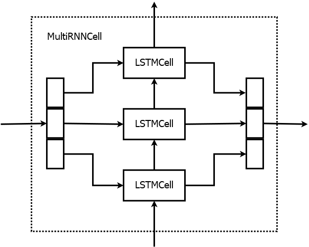 <!-- .element: class="plain" --> --- <!-- .slide: data-transition="none-in fade-out" --> ## RNNCell Wrappers * `DropoutWrapper(cell)` * Adds dropout. * `AttentionWrapper(cell, attention_mechanism)` * Implements attention over the decoder RNN `cell`. * Assumes we have the outputs of the encoder (memory). --- ## AttentionWrapper 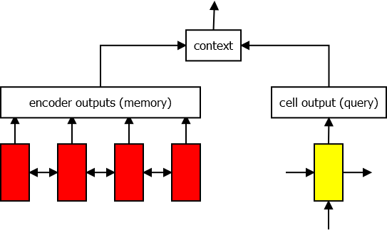 <!-- .element: class="plain" --> ```python decoder_cell = tf.nn.rnn_cell.LSTMCell(num_units) attention_mechanism = BahdanauAttention(num_units, encoder_outputs) attention_cell = AttentionWrapper(decoder_cell, attention_mechanism) decoder_outputs, _ = tf.nn.dynamic_rnn(attention_cell, decoder_inputs, final_encoder_state) ``` --- <!-- .slide: data-transition="fade-in none-out" --> ## Debugging * Assertion and print statements that need the actual value of the tensor should be added to the graph. * Problem: Assertion operation is not needed for computing the output. * The solution in TensorFlow: ```python assert_op = tf.Assert(tf.reduce_all(x > 0), [x]) x = tf.with_dependencies([assert_op], x) with tf.control_dependencies([tf.assert_equal(x, y)]): x = tf.identity(x) ``` * Printing is an identity operation that can be placed in the graph: ```python x = tf.Print(x, [tf.argmax(x)], 'argmax(x) = ') ``` --- ## TensorFlow Debugger * tfdbg can be used to debug problems that occur in the middle of training, e.g. inf values. * Run *n* steps or until some tensor values match a given filter. * Print values of tensors and trace them to Python code. * Display information about the computation graph. ```python from tensorflow.python.debug import LocalCLIDebugWrapperSession sess = LocalCLIDebugWrapperSession(sess) ``` ```python from tensorflow.python.debug import LocalCLIDebugHook ex = experiment.Experiment(..., train_monitors=[LocalCLIDebugHook()]) ``` --- ## Python Debuggers * There are many debuggers for Python: pdb, ipdb, pudb, ... * Enable by placing e.g. `import ipdb; ipdb.set_trace()` where you want to debug.  --- ## Custom Operation * `py_func` can convert a Python function into a TensorFlow operation. * Should take NumPy arrays as input and return NumPy arrays as outputs. * Print values, draw a plot using matplotlib, use Python debugger. ```python def debug_fn(x): print "x.shape={}".format(x.shape) if (x > 100).any(): import ipdb; ipdb.set_trace() return x output = tf.py_func(debug_fn, [input], tf.float32) ``` --- ## TensorBoard * The value of some variables can be monitored very easily during training. * In the code you only need to create a summary operation, for example: ```python tf.summary.scalar("mean_score", tf.reduce_mean(score)) ``` * Normally you would also need to collect the summaries and write to a log file using `tf.summary.merge_all()` and `tf.summary.FileWriter`, but Tensor2Tensor does this automatically. * TensorBoard is a web interface for monitoring training. * Start the service using `tensorboard --logdir <model directory> --port <port>` and point your web browser to the address that gets printed. --- ## TensorBoard – Scalars * The scalars page displays a graphical history of the scalar summary variables. 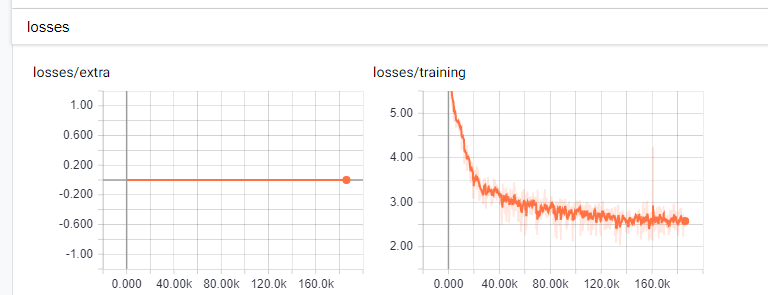 --- ## TensorBoard – Histogram * A histogram displays the distribution of a set of values. * The histogram is saved for the training step at specific intervals. ```python tf.summary.histogram("attention_peak", tf.argmax(alignments, 2)) ``` 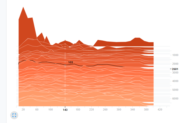 --- ## TensorBoard – Graph * The computation graph is also saved in text form in the model directory. * It can be inspected on the graphs page, showing the hierarchy in the variable and operation names. 